An Artificial Neural Network (ANN) is an information processing paradigm that is inspired by the biological nervous systems.

The key element of this paradigm is the novel structure of the information processing system. It is composed of a large number of highly interconnected processing elements (neurones) working in unison to solve specific problems.

Agenda

1. Learn basics of ANN
2. How Neural Net works
   • Perceptron
   • Neural Network Architecture
3. Learning Process of a Neural Network
   • Feed-forward Network
     • Single-layer Perceptron
     • Multi-layer Perceptron (MLP)
     • Convolutional Neural Network (CNN)
   • Reccurent Neural Network (RNN)

1. Basics of Artificial Neural Networks

ANNs, like people, learn by example. An ANN is configured for a specific application, such as pattern recognition or data classification, through a learning process. Learning in biological systems involves adjustments to the synaptic connections that exist between the neurones. This is true of ANNs as well.

The first artificial neuron was produced in 1943 by the neurophysiologist Warren McCulloch and the logician Walter Pits. But the technology available at that time did not allow them to do too much.

How Neural Networks Works?

To understand the working of a neural network we have to first understand

- Perceptron
- Architecture
- Learning Process

Perceptron

A Neural Network is combinations of basic Neurons — also called perceptrons arranged in multiple layers as a network.

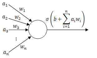
A neuron is a mathematical function that model the functioning of a biological neuron. Typically, a neuron compute the weighted average of its input, and this sum is passed through a nonlinear function, often called activation function, such as the sigmoid.

The output of the neuron can then be sent as input to the neurons of another layer, which could repeat the same computation (weighted sum of the input and transformation with activation function).

Note that this computation correspond to multiplying a vector of input/activation states with a matrix of weights (and passing the resulting vector through the activation function).

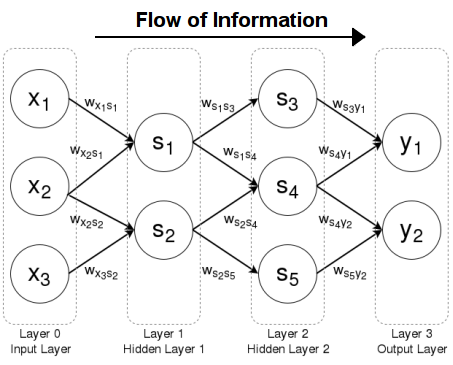
Artificial Neural Network Architecture

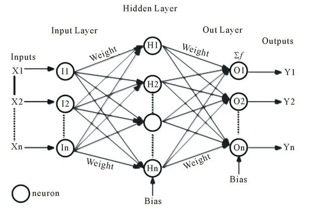
An Artificial Neural Network is made up of 3 components:

1. Input Layer
2. Hidden (computation) Layers
3. Output Layer

Input Nodes (input layer): No computation is done here within this layer, they just pass the information to the next layer (hidden layer most of the time). A block of nodes is also called layer.

Hidden nodes (hidden layer): In Hidden layers is where intermediate processing or computation is done, they perform computations and then transfer the weights (signals or information) from the input layer to the following layer (another hidden layer or to the output layer). It is possible to have a neural network without a hidden layer and I’ll come later to explain this.

Output Nodes (output layer): Here we finally use an activation function that maps to the desired output format (e.g. softmax for classification).

Connections and weights: The network consists of connections, each connection transferring the output of a neuron i to the input of a neuron j. In this sense i is the predecessor of j and j is the successor of i, Each connection is assigned a weight Wij.

Activation function: the activation function of a node defines the output of that node given an input or set of inputs. A standard computer chip circuit can be seen as a digital network of activation functions that can be “ON” (1) or “OFF” (0), depending on input. This is similar to the behavior of the linear perceptron in neural networks. However, it is the nonlinear activation function that allows such networks to compute nontrivial problems using only a small number of nodes. In artificial neural networks this function is also called the transfer function.

Learning Process of a Neural Network

For a neural network to work it is required to train it. training is when a neural network learns.

when neural networks are trained they process records one at a time, and “learn” by comparing their classification of the record (which, at the outset, is largely arbitrary) with the known actual classification of the record. The errors from the initial classification of the first record is fed back into the network, and used to modify the networks algorithm the second time around, and so on for many iterations.

A key feature of neural networks is an iterative learning process in which data cases (rows) are presented to the network one at a time, and the weights associated with the input values are adjusted each time. After all cases are presented, the process often starts over again. During this learning phase, the network learns by adjusting the weights so as to be able to predict the correct class label of input samples. Neural network learning is also referred to as “connectionist learning,” due to connections between the units. Advantages of neural networks include their high tolerance to noisy data, as well as their ability to classify patterns on which they have not been trained.

Question: So how does ANN adjusts weights and Biases to correct its predection?

Learning rule: The learning rule is a rule or an algorithm which modifies the parameters of the neural network, in order for a given input to the network to produce a favored output. This learning process typically amounts to modifying the weights and thresholds.

Applying learning rule is an iterative process. It helps a neural network to learn from the existing conditions and improve its performance.

Different learning rules in the Neural network: SEPERATE TUTORIAL FOR LEARNING RULES

1. Hebbian learning rule – It identifies, how to modify the weights of nodes of a network.
2. Perceptron learning rule – Network starts its learning by assigning a random value to each weight.
3. Delta learning rule – Modification in sympatric weight of a node is equal to the multiplication of error and the input.
4. Correlation learning rule – The correlation rule is the supervised learning.
5. Outstar learning rule – We can use it when it assumes that nodes or neurons in a network arranged in a layer.

Types of Neural Networks

1. Feed-forward Network
   • Single-layer Perceptron
   • Multi-layer Perceptron (MLP)
   • Convolutional Neural Network (CNN)
2. Reccurent Neural Network (RNN)

1. Feed-forward Networks: A feedforward neural network is an artificial neural network where connections between the units do not form a cycle. In this network, the information moves in only one direction, forward, from the input nodes, through the hidden nodes (if any) and to the output nodes. There are no cycles or loops in the network.

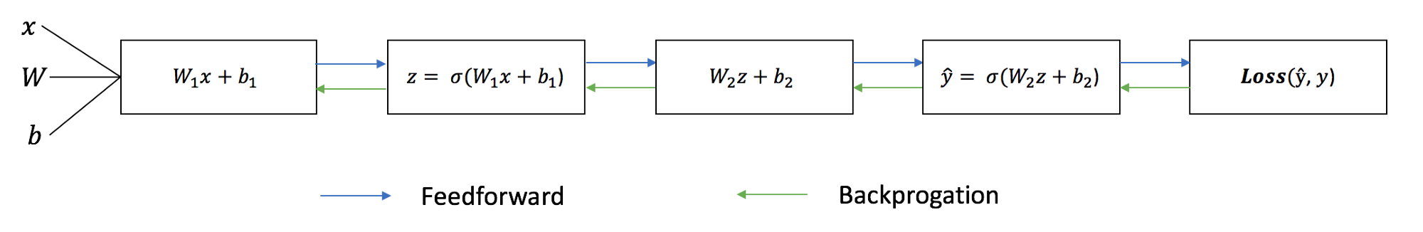
Each iteration of the training process consists of the following steps:

1. Calculating the predicted output ŷ, known as feed-forward
2. Updating the weights and biases, known as backpropagation

The sequential graph below illustrates the process.

Cost/Error/Loss Function

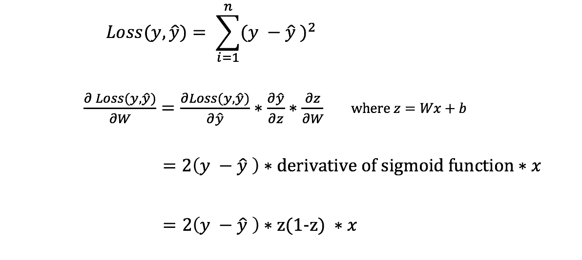
There are many available loss functions, and the nature of our problem should dictate our choice of loss function. In this tutorial, we’ll use a simple sum-of-sqaures error as our loss function.

That is, the sum-of-squares error is simply the sum of the difference between each predicted value and the actual value. The difference is squared so that we measure the absolute value of the difference.

Our goal in training is to find the best set of weights and biases that minimizes the loss function.

Some commonly used loss functions:

1. Qudratic Cost (Root Mean Square)
2. Cross Entropy
3. Exponential (AdaBoost)
4. Kullback–Leibler divergence or Information Gain

Backpropagation: short for “backward propagation of errors,” is an algorithm for supervised learning of artificial neural networks using gradient descent. Given an artificial neural network and an error function, the method calculates the gradient of the error function with respect to the neural network’s weights. It is a generalization of the delta rule for perceptrons to multilayer feedforward neural networks.

Once we’ve measured the error of our prediction (loss), we need to find a way to propagate the error back, and to update our weights and biases.

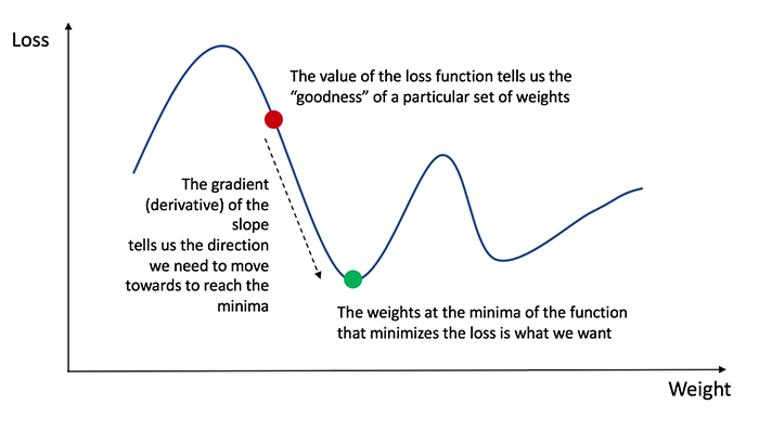
In order to know the appropriate amount to adjust the weights and biases by, we need to know the derivative of the loss function with respect to the weights and biases.

Recall from calculus that the derivative of a function is simply the slope of the function.

If we have the derivative, we can simply update the weights and biases by increasing/reducing with it(refer to the diagram above). This is known as gradient descent.

However, we can’t directly calculate the derivative of the loss function with respect to the weights and biases because the equation of the loss function does not contain the weights and biases. Therefore, we need the chain rule to help us calculate it.

Single-layer Perceptron: This is the simplest feedforward neural Network and does not contain any hidden layer, Which means it only consists of a single layer of output nodes. This is said to be single because when we count the layers we do not include the input layer, the reason for that is because at the input layer no computations is done, the inputs are fed directly to the outputs via a series of weights.

Multi-layer perceptron (MLP): This class of networks consists of multiple layers of computational units, usually interconnected in a feed-forward way. Each neuron in one layer has directed connections to the neurons of the subsequent layer. In many applications the units of these networks apply a sigmoid function as an activation function. MLP are very more useful and one good reason is that, they are able to learn non-linear representations (most of the cases the data presented to us is not linearly separable), we will come back to analyse this point in the example I’ll show you in the next post.

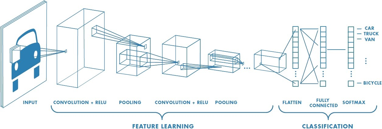
Convolutional Neural Network (CNN): Convolutional Neural Networks are very similar to ordinary Neural Networks, they are made up of neurons that have learnable weights and biases. In convolutional neural network (CNN, or ConvNet or shift invariant or space invariant) the unit connectivity pattern is inspired by the organization of the visual cortex, Units respond to stimuli in a restricted region of space known as the receptive field. Receptive fields partially overlap, over-covering the entire visual field. Unit response can be approximated mathematically by a convolution operation. They are variations of multilayer perceptrons that use minimal preprocessing. Their wide applications is in image and video recognition, recommender systems and natural language processing. CNNs requires large data to train on.

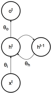
2. Reccurent Neural Network (RNN): In recurrent neural network (RNN), connections between units form a directed cycle (they propagate data forward, but also backwards, from later processing stages to earlier stages). This allows it to exhibit dynamic temporal behavior. Unlike feedforward neural networks, RNNs can use their internal memory to process arbitrary sequences of inputs. This makes them applicable to tasks such as unsegmented, connected handwriting recognition, speech recognition and other general sequence processors.